A twin study of GSCE results found that over half of the variance in grades could be attributed to genetic factors:
heritability was substantial for overall GCSE performance for compulsory core subjects (58%) as well as for each of them individually: English (52%), mathematics (55%) and science (58%). In contrast, the overall effects of shared environment, which includes all family and school influences shared by members of twin pairs growing up in the same family and attending the same school, accounts for about 36% of the variance of mean GCSE scores. The significance of these findings is that individual differences in educational achievement at the end of compulsory education are not primarily an index of the quality of teachers or schools: much more of the variance of GCSE scores can be attributed to genetics than to school or family environment.
While the shared environment is rather small relative to the genetic variance, we can consider how big a differences in scores you could make if you could magically change someone’s genes or environment but leave everything else about them the same.
First let’s look at the distribution of scores. I took numbers from main tables (XLS) in the 2013 results
EnglishGradeCount <- list(Astar = 20304, A = 68114, B = 126027, C = 174106,
    D = 94935, E = 42310, F = 16836, G = 5138)
MathsGradeCount <- list(Astar = 37075, A = 69429, B = 110726, C = 188947, D = 58911,
    E = 35678, F = 28273, G = 18912)
In the Shakeshaft et al study they coded the highest grade (A*) as 11 and and the lower (G) as 4
codings <- 11:4

plot(codings, unlist(EnglishGradeCount)/sum(unlist(EnglishGradeCount)), type = "h",
    xlab = "GCSE English score", ylab = "Frequency")

plot(codings, unlist(MathsGradeCount)/sum(unlist(EnglishGradeCount)), type = "h",
    xlab = "GCSE Maths score", ylab = "Frequency")

The results from the paper give the mean and SD of scores in their sample
englishMean = 8.93
englishSD = 1.17

mathsMean = 8.96
mathsSD = 1.4
and the heritabilities (called $h^2$ or $a^2$) and proportions of shared ($c^2$) and unique ($e^2$) environmental variance
englishA2 = 0.52
englishC2 = 0.31
englishE2 = 0.18

mathsA2 = 0.55
mathsC2 = 0.26
mathsE2 = 0.18
We can also calculate the weighted mean and SD from the 2013 data
EnglishScores <- cov.wt(matrix(codings), unlist(EnglishGradeCount))
MathsScores <- cov.wt(matrix(codings), unlist(MathsGradeCount))
sqrt(EnglishScores$cov)

##      [,1]
## [1,] 1.57
The combined genetic or shared environment effects are deviations from the mean with a standard deviation of $\sqrt{(v^2\sigma^2)}$ where $v^2$ is the proportion of variance and $\sigma^2$ is the variance (= the standard deviation squared). NB: I’m using the heritabilities from the study but the standard deviations and means from the 2013 results.
component_sd <- function(v2, sd) sqrt(v2 * sd^2)
# calculate genetic, shared environment, and unique environment standard
# deviations
englishASD <- component_sd(englishA2, sqrt(EnglishScores$cov))
englishCSD <- component_sd(englishC2, sqrt(EnglishScores$cov))
englishESD <- component_sd(englishE2, sqrt(EnglishScores$cov))
To make this concrete, think about drawing your GCSE scores from a genetic and environmental lottery. You start with the mean score, then pick a number from hats A, C, and E. The hats vary in size based on how much of the differences in scores each contributes. The bigger the hat (like the genetic hat, A), the farther from zero the numbers if yields will potentially be. With smaller hats, like the unique environment hat E, the numbers will be more clustered around 0. The numbers you get from the three hats are added or subtracted from the mean to produce your score.
set.seed(34450)
draw1 <- rnorm(3, mean = 0, sd = c(englishASD, englishCSD, englishESD))
draw1

## [1] -0.6979 -0.4289 -0.4988

EnglishScores$center + sum(draw1)

## [1] 6.507
So our first hypothetical person draws from the hat and gets 3 genetic, shared environment, and unique environment deviations that are below the mean (e.g., = ‘bad genes’, 'poor schooling’, 'bad experiences’). These add up to a GSCE score of 6.5 (between an E and a D)
draw2 <- rnorm(3, mean = 0, sd = c(englishASD, englishCSD, englishESD))
draw2

## [1]  1.1156 -0.5552  0.7212

EnglishScores$center + sum(draw2)

## [1] 9.414
The next person gets positive genetic and unique environment deviations but a negative shared environment deviation (= 'good genes’, 'poor school’, 'good experience’). These factors combine together to result in a score of 9.4 (a B).
We can look at the distribution of deviations on each of these factors in comparison to the phenotypic variance (P)
scores <- seq(4, 11, by = 0.01)
englishADensity <- dnorm(scores, mean = EnglishScores$center, sd = englishASD)
englishCDensity <- dnorm(scores, mean = EnglishScores$center, sd = englishCSD)
englishEDensity <- dnorm(scores, mean = EnglishScores$center, sd = englishESD)
englishPDensity <- dnorm(scores, mean = EnglishScores$center, sd = component_sd(1,
    sqrt(EnglishScores$cov)))
plot(codings, unlist(EnglishGradeCount)/sum(unlist(EnglishGradeCount)), type = "h",
    xlab = "GCSE English score", ylab = "Frequency", ylim = c(0, 0.6))
lines(scores, englishADensity, col = "blue")
lines(scores, englishCDensity, col = "orange")
lines(scores, englishEDensity, col = "red")
lines(scores, englishPDensity, col = "purple")
legend("topright", c("A", "C", "E", "P"), col = c("blue", "orange", "red", "purple"),
    lwd = 3)
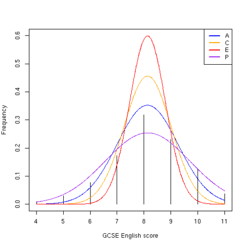
The plot shows the distribution of deviations around the mean for each of the factors compared to the phenotypic variance (purple). If your genetic (blue) and shared environment (orange) factors are average (with values of 0), then your unique environment deviation could not move you very far from the mean. This is what the paper means when it says that the unique environment contributes very little to the variance. The genetic factor, in contrast, is more spread out, so having genes that contribute very positively or very negatively to your score can move you far away from the mean.
Yet the environent can still make a big difference to test results if we were able to manipulate it. For example, if we took someone whose genetics and individual experience were average and moved them into a great family/school environment (2SD above the mean), we could potentially raise their English GCSE score from an 8 (a C) to a $8 + 2 \times \sqrt{.31 \times 1.6^2} = 9.8$ (which is almost an A). A student’s whose genes predispose them to the high intelligence and motivation that would result in an A* could be pulled down to a B by an unsupportive family/school environment. And someone’s whose genetic endowment destines them for a G could be potentially pulled up to a $4 + 2 \times \sqrt{.31 \times 1.6^2} + 2 * \sqrt{.18 \times 1.6^2} = 6.7$ (an E) with the right mix of interventions.
patchworkjukebox reblogged this from differential
differential posted this