isomorphismes

If you’re using base::plot in R for the first time you may have looked at ?plot (2 page help file) or ?par (12 page help file) to figure out what’s going on. It’s overwhelming.

This document explains the parameters I always bother to set. That way you can get decent plots without reading every parameter’s description.

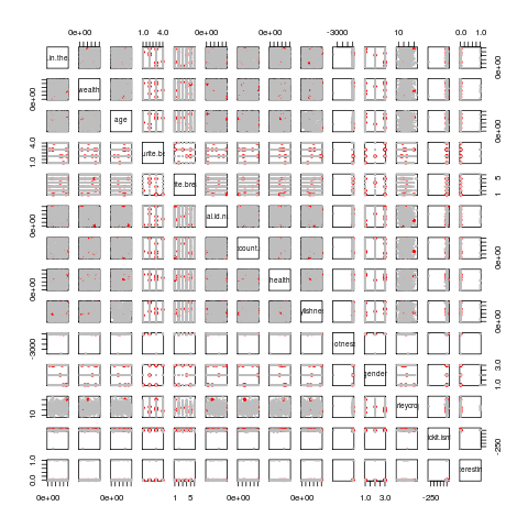
(If you are just using R for the very first time and need some data, type data(faithful) or data(pima) to load some interesting pre-cleaned data sets. Then do plot(pima) or plot(faithful) to see how the base::plot functions. Type ??pima if you can’t find the dataset.) 

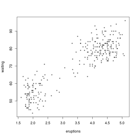
> plot(faithful, pch=20, col=rgb(.1,.1,.1,.5), cex=.6)

Firstly: what is par? When you type par( lwd=3, col="#333333", yaxt="n" ), it will open an empty box that will hold your next plot( dnorm, -3, 3). You can run different plots in the box and as long as you don’t close it, the line-width will be 3 times bigger than default, the y-axis won’t have labels, and the colour will be dark-grey.

There are a lot of plotting options. Here are the ones I use regularly:

• cex = .8. Decreases the size of type or plotted points by 20%.
• par(new=TRUE). Use this to plot two things on top of each other. Beware, the labels will overprint over each other too (but this doesn’t matter for quick, casual plots).
  
   
• col = "red", col = "#333333". I think #333333 is the best default colour and I use red if a point or line needs to stand out.
   
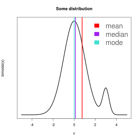
• col=rgb(.1,.1,.1,.5). This is another decent grey for overplotting. I used this in the Old Faithful plot at the top. The first three numbers are Red, Green, Blue and the fourth is Transparency.
• lwd = 3. This is a good line width, I think, especially with the dark grey col="#333333".
• pch = 20. Plots points with a small circle. pch=19 is a slightly larger dot and pch=15 is a square. Read after the second group of bullets for more info.
• png("name of the plot.png"). Then do plot(x), par(new=TRUE), plot(y), par(new=TRUE), plot(z), and remember to finish it off with dev.off(). [dev.off() means device off; the par() window and the png() file are considered “graphic devices”.]

Here are the ones I use less regularly, but still more than weird stuff like oma, mex, mai, etc.

• lend = butt. Line ending is square rather than mitred. I use this before I make a histogram.
• ylog=TRUE, xlog=TRUE. “Hubble made this significantly worse chart before it was discovered that all data look like straight lines on log-log plots.” –Lawrence Krauss
• las=1. If you want all of your axis labels to be printed horizontally.
• mfrow=c(2,2). If you want to juxtapose four plots next to each other. mfrow and they will write like a typewriter, left-to-right and starting over on a new line after 2 spots have been filled in. mfcol=c(3,3) and they will fill in vertically. (Try it if what I said doesn’t make sense.)
• yaxs="n". This suppresses printing the vertical axis labels. I do this when plotting a distribution because those vertical numbers aren’t meaningful.
• main="It's a plot about nothing. Don't you get it? People _love_ nothing!". This is the title of the plot.
• legend( "top right", legend=c("control", "placebo", "test group"), fill = c("black", "#333333", "red"), border="white", bty="n"). This is how I find legends look good. You should only need to change the placement, legend text, and fill to make it work for your plot.
• To plot multiple figures in the same picture do mfrow=c(3,2) or mfcol=c(3,2). Then the next six = three × two plots you run will go in left-to-right or up-to-down order, filling in six spots.
  
  Don’t forget to do par(mfrow=c(1,1)) after you’re done, to go back to one plot per diagram.
• If you want to save your plot to a file rather than “print” it to the screen, type png("a plot about nothing.png"); plot( stuff ); dev.off(). The dev.off() tells the system to go back to normal (printing to the screen–PNG device off).
• One more awesome  advice from the StackOverflow R community: how to get some sweet, sweet log-axis tickmarks. Read all about it.

Most of these can be done inside of plot( dpois, 0, 15, lwd = 3) or beforehand in a par(lwd=3); plot( dpois, 0, 15). With par(new=TRUE) and par(mfrow=c(2,2)), though, you need to do them in a par() beforehand.

If you forget what the colours or the pch shapes are, do this: plot( 1:25, pch=1:25, col=1:25 ). You’ll get this:

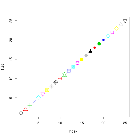
So basically, you only want pch=20 and sometimes pch=19 or pch=15, like I said.

One more thing you might like to learn is how to colour important data points red and normal ones grey. I’ll explain that another time.