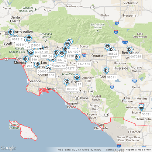
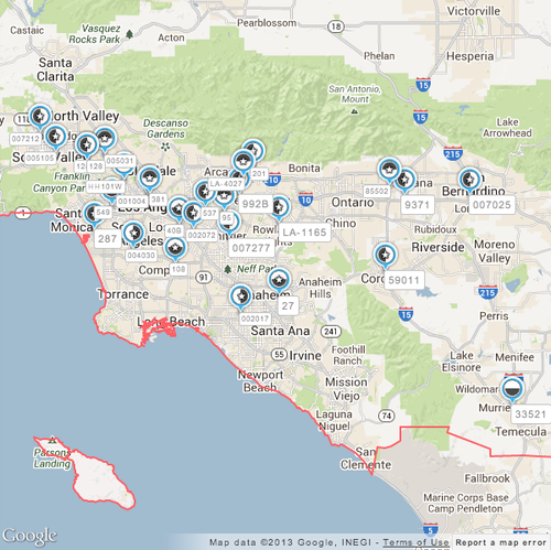
After having pruned proposals for an RFP, our agency users often require a PowerPoint presentation export of the chosen inventory to present to their client. Our software enables them to do so, generating within seconds a PowerPoint that usually takes them hours to put together by hand. These PowerPoints contain maps detailing inventory locations in all the relevant markets, inventory photos, pricing and other relevant information. Recently, one of our users requested us to include labels containing unit numbers for the inventory markers in the coverage maps. Since proposed inventory within a market can often be located very close together, we had to come up with a strategy for labeling these markers while reducing the overlap amongst them so as to maximize readability. Here is a screenshot of a map with inventory labelled but not optimized for readability:
We ended up experimenting with two (local) search AI algorithms to optimize label sizing and placement for maximizing readability. AI search algorithms are used to find optimal solutions to problems that can be modeled in terms of discrete states, and a transition function that can produce allowed (neighboring) states when given a state and a legal transition as input. The set of allowed states for a problem formulates its search space. The algorithm has to traverse the search space efficiently and arrive upon a state that optimizes a pre-defined objective function. Brute-force search algorithms like Depth-first Search and Breadth-first Search are too inefficient to be able to solve problems that have large search spaces.
For the map-marker labeling problem, the objective function that we chose to minimize was the total label overlap (measured in square pixels). A state, in the context of this problem, refers to a map with a certain number (say, n) of labeled markers. Further, a neighboring state is produced by moving a label on any one marker to a different position. Since we allow 10 different positions for a map-marker label, our transition function can produce 10n neighboring states for any given input state (also know as the branching factor). Our search space consists of 10^n states. For 50 markers, the search space has more states than the number of stars in the universe (10^24)! Here are screenshots of the 10 different positions that we implemented for a label on a marker:
The labels have a maximum width of 110px. The large ones have a height of 21px (11px font) and the smaller ones are 14px high (8px font).
The first search algorithm that we experimented with, Hill Climbing, is a greedy algorithm which when applied to our problem, can be summarized in the following steps:
Given an initial state, pick any two labels that overlap.
Move one of the labels to a position that reduces the total label overlap.
Set the resulting state as the initial state.
Repeat steps 1-3 until the overlap has been reduced to zero or a certain number of iterations have been run.
The second algorithm, Simulated Annealing, is a stochastic search algorithm. It can be summarized in the following steps:
Given an initial state, pick any two labels that overlap.
Move one of the labels to a random new position.
Set the resulting state as the initial state with a probability of where is the difference in “system energy" (total label overlap) between the resulting state and the prior state and T is the cooling schedule (explained below).
Repeat steps 1-3 until the overlap has been reduced to zero or a certain number of iterations have been run.
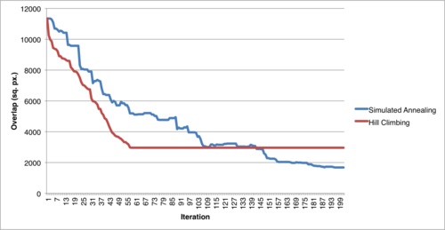
Our experimentation methodology was as follows – n markers were placed randomly on a map of size 450px by 450px (the size of the maps in our PowerPoint exports) and the value of n was set to 10, 20, 30, 40, 50 and 60. For each value of n, we ran the experiment 30 times to reduce the bias of any individual run. For each random placement, we ran both algorithms (with a maximum of 200 iterations each) and measured the percentage reduction in label overlap. The average overlap reduction was calculated for both algorithms for each setting of n. The results are presented in the following graph:
The Simulated Annealing algorithm outperformed Hill Climbing by an overall margin of 17% (absolute). As expected, we observed that the latter would often get stuck in local minima – unable to find a globally optimal solution. The former, on the other hand, because of its stochastic nature was able to explore a much larger fraction of the search space and return a minimum that if not globally optimal, was almost so. The following graph which shows data from one of our runs with a map with 50 markers illustrates this point well:
In this case, even though the greedy Hill Climbing algorithm is able to reach a minimum faster, it gets stuck there – unable to find a neighboring state with a lower value of the optimization function to move to. The Simulated Annealing algorithm does not always pick a state with a lower value of the optimization function (as can been seen by the intermittent spikes in the graph) but is eventually able to navigate to a more optimal solution.
Affect of Cooling Schedule on the Performance of Simulated Annealing:
The cooling schedule (T) essentially determines how fast the randomness in the Simulated Annealing algorithm decreases. An ideal cooling schedule has a T that is high when the algorithm starts so that it accepts states with higher “energy" with greater probability. As the algorithm proceeds, and it gets closer to discovering the global minimum, the value of T should reduce so that transitions are made only to states that have lower energy. Consider the following analogy – if you try getting a ball to the lowest point in a box containing a solid material that forms peaks and valleys in the box, you could shake the box vigorously at first (high T), getting the ball to bounce around randomly. As the ball starts entering low valleys you reduce the shaking and let gravity take over (low T), getting the ball to roll into the lowest valley on it’s own.
A variety of functions can be used for T – exponential, logarithmic, oscillating etc. The choice of a cooling schedule function is very specific to the problem at hand. Thus, we performed an experiment in order to determine the optimal cooling schedule for our problem. We generated 30 maps, each with 50 map markers placed randomly and ran Simulated Annealing with seven different cooling schedules on each one. We chose a mix of functions with a variety of slopes and periods. The seven functions were:
Linear:
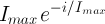
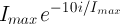
Exponential-1:
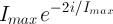
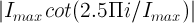
Exponential-2:
Logarithmic:
Cotangent:
Periodic-Exponential-1:
Periodic-Exponential-2:
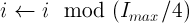
Where
is the maximum number of iterations for a run of the algorithm (which we set to 200) and is the current iteration number (1 through 200). The periodic exponential functions involve 4 periods of the exponential function (we perform the following assignment before calculating the value of the function: ). All seven functions are plotted in the following graph:
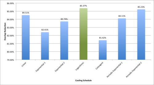
The results obtained from this round of experiments are summarized in the following graph:
The logarithmic function outperformed the others, achieving an average overlap reduction of 85.37% over the 30 runs. The Periodic-Exponential-2 function was a close second with an average overlap reduction of 85.23%. It seems like the algorithm performs best with a schedule that has a high value to start and then decays very quickly (i.e. large slope). The logarithmic function fits the bill. The periodic exponential functions also perform decently well, especially Periodic-Exponential-2. It has high slope, and because it is periodic, it causes the algorithm to discover at least 4 (the number of periods in the function), possibly different, minima. The minima that is the least of the ones discovered can be used as the solution.
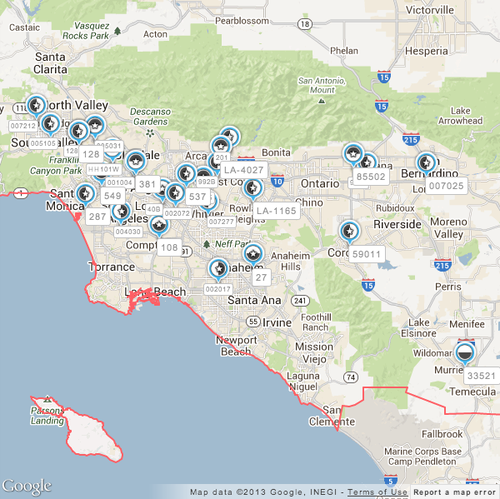
Finally, here is the result of running Simulated Annealing with the Logarithmic cooling schedule on the map shown above (overlap reduction of 97%):
And here is the result of running Hill Climbing on the same map (overlap reduction of 84%):
The first one clearly has more unobscured labels, and is more readable.
We were successfully able to apply two search (optimization) algorithms from AI literature on the map-marker labeling problem. Even though the results are specific to our setting, we believe that the Simulated Annealing algorithm would perform well in a generic point-labeling setting.
Learn about the technology behind ADstruc, from the people who create it.
ADstruc is the leading buying platform for the outdoor advertising industry, including both traditional and digital Out-of-Home media.
With an emphasis on data-driven planning, we help agencies, national brands, and local businesses discover and efficiently purchase Out-of-Home media campaigns that deliver tangible and measurable results.
Our cloud-based solution also allows outdoor advertising vendors to easily manage their inventory online and interact with new and existing clients in real-time.